
The Risk is in the Tail: Planning for Losses from Natural Disasters
How much capital should be set aside to adequately meet anticipated disaster-related losses across U.S. states?

Natural disaster relief has become an increasingly critical and contested topic. Evidence from recent studies and news coverage points to significant underinsurance in real estate markets. At the same time, there is renewed discussion about the respective responsibilities of federal and state governments in disaster response and recovery.
This post addresses a fundamental question: how much capital, combining resources from insurance, state relief, and federal relief, should be set aside for each state to adequately meet anticipated disaster-related losses?
Falling short of the capital required to address losses can have severe consequences for the local population and economy, and lead to slow and problematic recoveries. However, overcommitting resources is also problematic, especially when state and federal funds are involved. It may delay or prevent the implementation of other essential projects.
The central point we would like to stress is that regulators, when determining capital needs, should focus not only on “mean” expected losses, but on the entire distribution of potential losses. Focusing solely on the mean expected loss may leave U.S. states underfunded in many reasonably likely scenarios.
For example, the 2023 FEMA’s National Risk Index (NRI) dataset provides estimates of the expected annual loss for each U.S. county from disasters such as floods, hurricanes, and wildfires. Aggregating expected annual hurricane-related losses across all Florida counties yields a total estimated expected loss of $7.2 billion for buildings (real estate). However, in 2024, two major hurricanes (Helene and Milton) struck the state, causing over $30 billion in property damage. This stark disparity highlights how resources calibrated to cover only the expected loss can fall dramatically short in the face of severe disasters. At the same time, Helene and Milton might have been extreme events, and it is unreasonable to set budget goals based on extremely rare occurrences.
We propose here a middle ground, which is to estimate the minimum amount of capital required to cover losses that are infrequent, but not highly unlikely. For example, those with 1-in-10 (10%) or 1-in-20 (5%) annual probability. This is the Value-at-Risk (VaR) methodology, widely used in finance and insurance.
We find that the “right tail” of the distribution of disaster losses is long, and VaR estimates, capturing the capital needed to cover infrequent, but not improbable, events substantially exceed “mean” expected losses. This is especially true for wildfires, which tend to have low expected annual loss, but comparatively really large VaR.
The Value-at-Risk (VaR) Approach
The Value-at-Risk (VaR) approach provides a quantitative assessment of the minimum amount of capital needed to meet losses from events that occur with probability smaller or equal than p, which is is the Value-at-Risk threshold.
Calculating VaR involves two main steps. First, one must derive the distribution of losses. This can be done either analytically or through simulation. Second, a risk threshold p is selected, commonly set at 10%, 5%, or 1%. As shown in the figure below, the 5% VaR corresponds to the 95th percentile of the loss distribution (the loss amount that is exceeded only by the highest 5% of outcomes).
We construct annual state-level loss distributions by running simulations based on county-level data from the 2023 FEMA’s National Risk Index (NRI). This dataset provides the probability of various disasters and the expected losses to buildings conditional on a disaster occurring.1 A key assumption in our simulation is that disaster occurrences are uncorrelated across counties. To the extent that disasters are instead spatially correlated, our approach will underestimate the upper tail of the loss distribution, and thus the VaR amount. Moreover, conditional on a disaster striking, we do not model the occurrence of extreme losses. Thus, our VaR estimates should be interpreted as conservative. We focus on losses from hurricanes and wildfires, which have been particularly devastating types of natural disasters in the last decades.
The Distribution of Losses in Florida and California
The figures below report the simulated distribution of the dollar amount of building losses for Florida, the state most exposed to hurricanes, and California, the state most exposed to wildfires.
Starting with Florida, the distribution of losses is highly dispersed, with a long “right tail” representing scenarios involving large-scale damage. The red and magenta lines indicate the 10% and 5% Value-at-Risk (VaR) levels, corresponding to losses of $10.2 billion and $11.3 billion, respectively. This implies that Florida faces a 1-in-10 chance of incurring annual losses of $10 billion or more, and a 1-in-20 chance of losses of $11 billion or more. These figures stand in stark contrast to the expected loss (black line) of approximately $7.2 billion.
Calibrating capital resources to just meet the expected loss can leave disaster recovery substantially underfunded with relatively high likelihood.

This point becomes even more striking when we examine the distribution of wildfire-related losses in California. Unlike the hurricane loss distribution in Florida, most simulated scenarios for California involve minimal losses. However, the right tail of the distribution is extremely long, encompassing rare but catastrophic events.
The intuition is that fires occur far more frequently in areas with limited exposed real estate. However, when fires do strike regions with significant property exposure, they can result in substantial losses. Extreme examples are the fires in Pacific Palisades and Altadena.
As a result, the expected loss provides in this context even less guidance than in the case of hurricanes.
The black line marks an expected annual loss of $1.4 billion. In contrast, the 10% Value-at-Risk is $3.8 billion, and the 5% Value-at-Risk soars to $12.2 billion. This implies that California faces a 1-in-20 chance of incurring wildfire losses nearly ten times the expected loss amount in a given year.

Value-at-Risk from Hurricanes and Wildfires across U.S. States
We extend the analysis beyond Florida and California to include all states with substantial exposure to hurricane or wildfire risk. The table below reports the top 20 states ranked by expected loss from hurricanes. For each state, we show the expected loss, along with Value-at-Risk (VaR) estimates at the 10%, 5%, and 1% thresholds.
Florida, Texas, North Carolina, South Carolina, and Louisiana have the highest expected losses as well as the highest VaR figures across all thresholds. Among these states, the 5% VaR exceeds the expected loss by 50% to 200%, with the largest gap observed in Texas. At the 1% VaR level (a more conservative benchmark) Florida would require $13 billion in capital, while Texas would require nearly $9 billion. Even when using the 5% threshold, capital needs exceed $1 billion in each of the top 15 states.

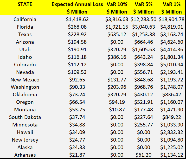
The table below presents the same analysis for wildfire risk. The gap between expected loss and VaR is even more pronounced than in the case of hurricanes. California is the only state with expected annual wildfire loss exceeding $1 billion. In contrast, Florida and Texas (the second and third most exposed states) have expected loss of less than $300 million. However, Florida has a 5% VaR of $3 billion, and Texas $1.2 billion. This again highlights that capital reserves based solely on expected loss would be inadequate for covering even moderately unlikely events.
Similar effects are observed in Arizona and Utah, where the expected loss is below $200 million, but the 5% VaR reaches $600 million and $1.6 billion, respectively. Additionally, some states such as Colorado and Hawaii appear relatively unexposed even under likely tail scenarios, with low 10% and 5% VaR, but face the potential for extreme losses in rare events. Colorado, for instance, has a 1% VaR of $5 billion, while Hawaii’s 1% VaR exceeds $1 Billion.
Conclusion
We believe that Value-at-Risk analysis, and more broadly, examining the right tail of loss distributions, is a valuable tool for agencies involved in planning and allocating resources for natural disasters.
The specific figures in our analysis are subject to some limitations. They rely on statistical approximations and on FEMA estimates published in 2023, which may be revised as new data on climate risk become available.
While the exercise presented here is a simplified example based on readily available data, it illustrates how such methods can offer a more realistic picture of disaster risk exposure and inform more resilient funding strategies.
Our simulation is constructed using the public data from FEMA NRI. We simulate the distribution of annual losses by randomly assigning disasters to each county, using the estimated county-level probabilities from FEMA’s data, over 250,000 draws. If a disaster does not occur, the loss is set to zero. If a disaster does occur, the loss is equal to the expected building loss (calculated by FEMA as the value of exposed buildings multiplied by the historical loss ratio) plus a lognormal shock. This shock reflects the fact that realized losses can deviate from their expected values. While we were unable to calibrate this shock empirically, we assume a standard deviation of 10% in this calculation. This value likely understates the true degree of uncertainty surrounding expected losses.