
Neighborhood Analysis with Housing Data and Machine Learning
We develop a data-driven approach to classify homes, and use it to identify neighborhood features and trends in LA County

Tracking neighborhood transformation within a city is important for several reasons. It helps investors and local policymakers identify areas undergoing gentrification, or neighborhoods that have fallen behind amid broader urban change. It can also enable regulators to more effectively target incentives to stimulate localized real estate development. However, accurately assessing a neighborhood’s situation is not straightforward and may require highly detailed information on local residents.
In this post, we propose an approach that leverages the characteristics of the local real estate market. Using detailed data on single-family parcels, we (1) cluster the existing housing stock into quality tiers based on structural attributes (age, size, etc.), and (2) analyze which clusters dominate in each neighborhood. This allows us to identify transforming areas, neighborhoods that have been overlooked by redevelopment, and those that have benefited from recent new construction.
We apply our method to Los Angeles County and demonstrate that it can be easily used to categorize local single-family homes into distinct types, and to develop a straightforward definition of transforming/gentrifying areas that is strongly correlated with recent price growth. Intuitively, transforming areas can be identified by a mix of homes belonging to the highest and lowest quality buckets within the metropolitan area.
Defining “Home Types“
We want to categorize single-family homes within a metropolitan area into distinct “home types”, based on their physical characteristics. We intentionally exclude location from the classification because our aim is to use the attributes of the housing stock to help differentiate neighborhoods within the city. Defining home types is a complex problem: How many categories should there be? Should homes be grouped by age, size, or some combination of features?
For our analysis, we adopt the following approach. First, we select four key physical characteristics that reflect the appearance and structure of a home:
Effective Year Built: This is not the original construction year of the building, but rather a date that reflects the current structure and wear-and-tear of the home. For example, a house initially built in 1960 but heavily renovated in the early 2000s could have an effective year built of 2000, indicating that its current state aligns more closely with a newer property.
Number of Bedrooms
Living Square Feet: This is the size of the interior space of the home.
Living Square Feet Divided by Lot Size: This is the ratio of the interior space of the home to the lot size. It reflects how intensively the lot has been developed.
Second, based on these characteristics, we cluster homes using the k-means algorithm, which is a widely used machine learning technique for unsupervised classification. Given a set of features, k-means assigns each observation to one of k clusters, grouping together observations that are similar across all dimensions. In this context, homes within the same cluster share comparable physical attributes. We apply this method to Los Angeles County, using approximately 1.39 million observations on single-family parcels as of the end of 2022.
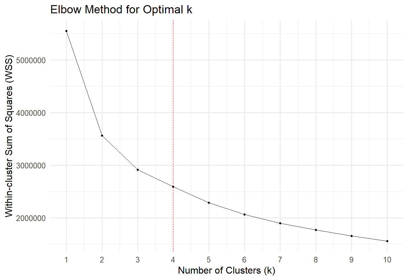
Mechanically, increasing the number of clusters improves the fit of the k-means algorithm. To select a parsimonious number, we apply the Elbow rule, which recommends choosing the smallest number of clusters beyond which additional clusters yield diminishing improvements in fit. The figure below illustrates this using the within-cluster sum of squares, a standard measure of fit that captures the similarity of observations within each cluster. Lower values of the black line indicate a better fit. We choose to use four clusters, because the curve flattens noticeably after four clusters, suggesting that additional clusters offer only marginal gains.
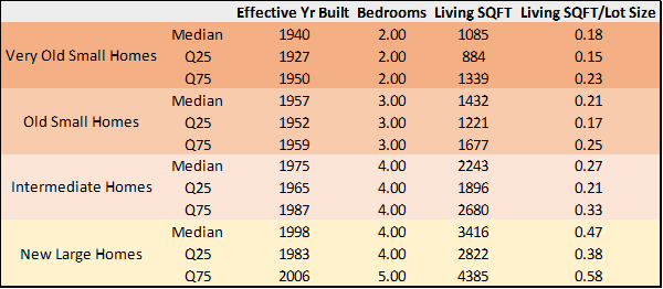
Interestingly, the algorithm produces a highly intuitive grouping of properties, making it easy to interpret each cluster as a distinct type of home. The table below summarizes the characteristics of homes in each cluster. We define them as:
Very Old Small Homes (296,226 observations, or 21.34% of homes): The first cluster mainly consists of homes that have an effective year built between the 1920s and the 1940s, 2 bedrooms, and living square feet between 880 and 1340. These houses also tend to occupy a smaller share of their lot, with living square feet equal to 15-20% of the lot size.
Old Small Homes (99,681 observations, or 7.18% of homes): This is the smallest cluster, comprising homes that are slightly more recent, with an effective year built in the 1950s, and slightly larger, with 3 bedrooms and living square footage between 1,200 and 1,700.
Intermediate Homes (644,179 observations, or 46.41% of homes): This is the largest cluster, consisting of homes built in the 1970s and 1980s, with 4 bedrooms and living areas ranging from approximately 1,000 to 2,000 living square feet. Interestingly, these homes utilize their lots more effectively, with living square footage equal to 20-30% of the lot size.
New Large Homes (347,802 observations, or 25.06% of homes): This is the most modern group, comprising properties built in the 1990s and 2000s, and thus also including newly built properties. They are larger than homes in other clusters, with 4 or 5 bedrooms, living areas ranging from the high 2,000 to above 4,000 square feet, and they occupy a large share of their lots, between 40% and 60%.
Los Angeles Neighborhoods with a Prevailing Home Type
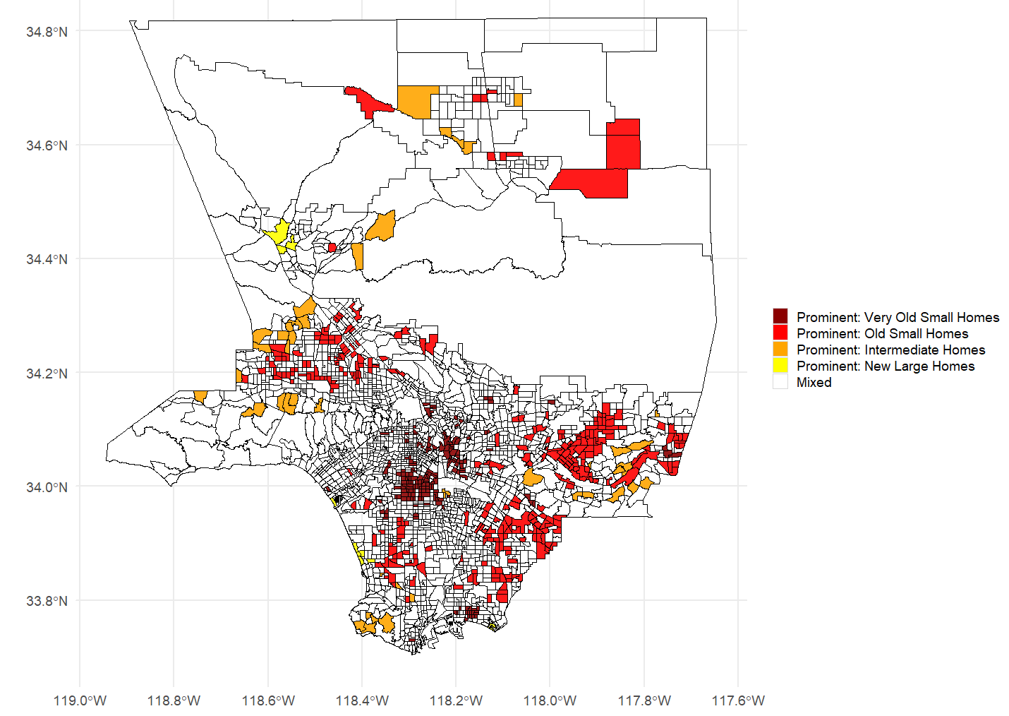
With the home type clusters defined, we can now use them to describe neighborhood composition across Los Angeles County. The figure below divides the county into Census tracts and highlights those in which a single cluster is prevalent, meaning it accounts for more than 50% of the homes in the tract, while no other cluster exceeds 20%. This allows us to identify neighborhoods dominated by a distinct home type.1
The dark red areas represent neighborhoods where Very Old Small Homes are prevalent. These areas are primarily located south and east of Downtown Los Angeles, and are neighborhoods where housing quality has lagged behind that of the broader metropolitan area. A similar prevalence of Very Old Small Homes is also present in parts of Long Beach. Old Small Homes are prevalent in several neighborhoods in the eastern portion of the county and throughout the San Fernando Valley. New Large Homes are prevalent only in a handful of neighborhoods, typically in the more affluent locations, such as Venice, Manhattan Beach, and Redondo Beach.
Transforming (Gentrifying) Neighborhoods
An even more insightful application of our classification is identifying neighborhoods that have been or are actively undergoing transformation and potentially gentrification.
Intuitively, the most striking cases of transformation should coincide with areas that currently or historically had a large share of Very Old Small Homes and Old Small Homes, but have since seen redevelopment, with many properties replaced by New Large Homes. We identify such neighborhoods as Census tracts in which New Large Homes is the most or second most frequent type, but the other most frequent type is either Very Old Small Homes or Old Small Homes.
The figure below highlights 64 Census tracts that fit these criteria, located within the core metropolitan area of the county.
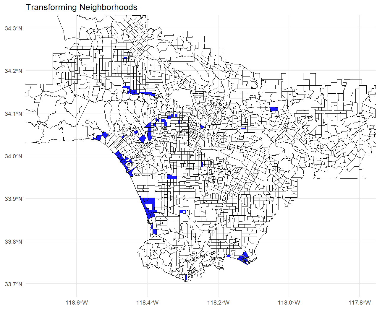
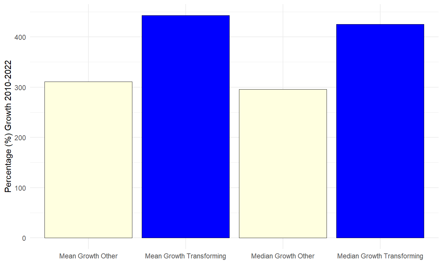
Consistent with our hypothesis that the transforming neighborhoods identified by our approach are gentrified or gentrifying, we find that these areas have experienced significantly higher house price growth than the rest of Los Angeles County over the past decade. To quantify this, we calculate house price growth at the Census tract level using data on home values from the American Community Survey (ACS) for the years 2010 and 2022. We compare mean and median house price growth in the Transforming Census tracts identified by our approach to those in the rest of the county. While Census tracts outside these areas also experienced substantial appreciation, with average price growth exceeding 300% between 2010 and 2022, the Transforming tracts saw even faster increases, with both mean and median growth exceeding 400% (one-third higher than that of other tracts).
Conclusion
It is crucial for investors and regulators to develop a bird’s-eye view of neighborhood disparities within metropolitan areas, as well as emerging trends in transformation and gentrification.
We demonstrate that a simple machine learning approach can be highly effective in identifying these patterns. It provides an interpretable classification of the local housing stock into distinct types and characterizes neighborhood composition.
Broadly, the single-family housing stock can be grouped into old, small homes and large, new homes. The coexistence of the oldest and newest home types within the same neighborhood signals active transformation and is associated with rapid house price growth.
We restrict our analysis to Census tracts with more than 50 single-family homes.