
The Wired-Internet Gap Across U.S. Counties
The county-level share of households with wired home internet varies dramatically, from 16% to 97%. We explore how the gap relates to local income, education, school quality, and geographic isolation.

Universal home internet has been a stated U.S. policy goal for over fifteen years, starting with the 2010 National Broadband Plan and the Connect America Fund, and continuing most recently with the Emergency Broadband Benefit and Emergency Connectivity Fund, both launched during the COVID-19 pandemic.
These efforts are based on the premise that a high-quality home internet connection is an incredibly valuable resource, providing access to a wide range of services, information, and opportunities. Access matters even more for lower-income and rural communities, where local services and opportunities are more limited and a fast connection can act as an important equalizer. Moreover, with the rise of large language models and other powerful internet-distributed tools, access to fast and reliable internet is likely to become even more valuable in the years ahead.
Until recently, there were no official estimates of differences in wired-internet connections across U.S. counties. The Census has run a periodic survey since 1994 on behalf of the National Telecommunications and Information Administration (NTIA), collecting information on wired internet adoption. However, the survey can be used for representative estimates only at the national or state level.
In 2024, the Census Bureau launched the Local Estimates of Internet Adoption (LEIA) product. These are model-based projections for year 2022, which combine the NTIA’s survey with American Community Survey restricted microdata and other sources (such as FCC Broadband Data). They provide estimates of county-level wired-internet adoption, which is defined as the share of households with wired-internet at home.
In this post, we explore the data and document staggering variation across counties both within and across states, which is correlated with socioeconomic characteristics, geography, and school quality. Overall, adoption is lowest in areas with lower incomes, weaker schools, and greater geographic isolation. These locations would likely benefit greatly from widespread reliable home internet, yet they appear to have been left behind.
The Gap Across U.S. Counties
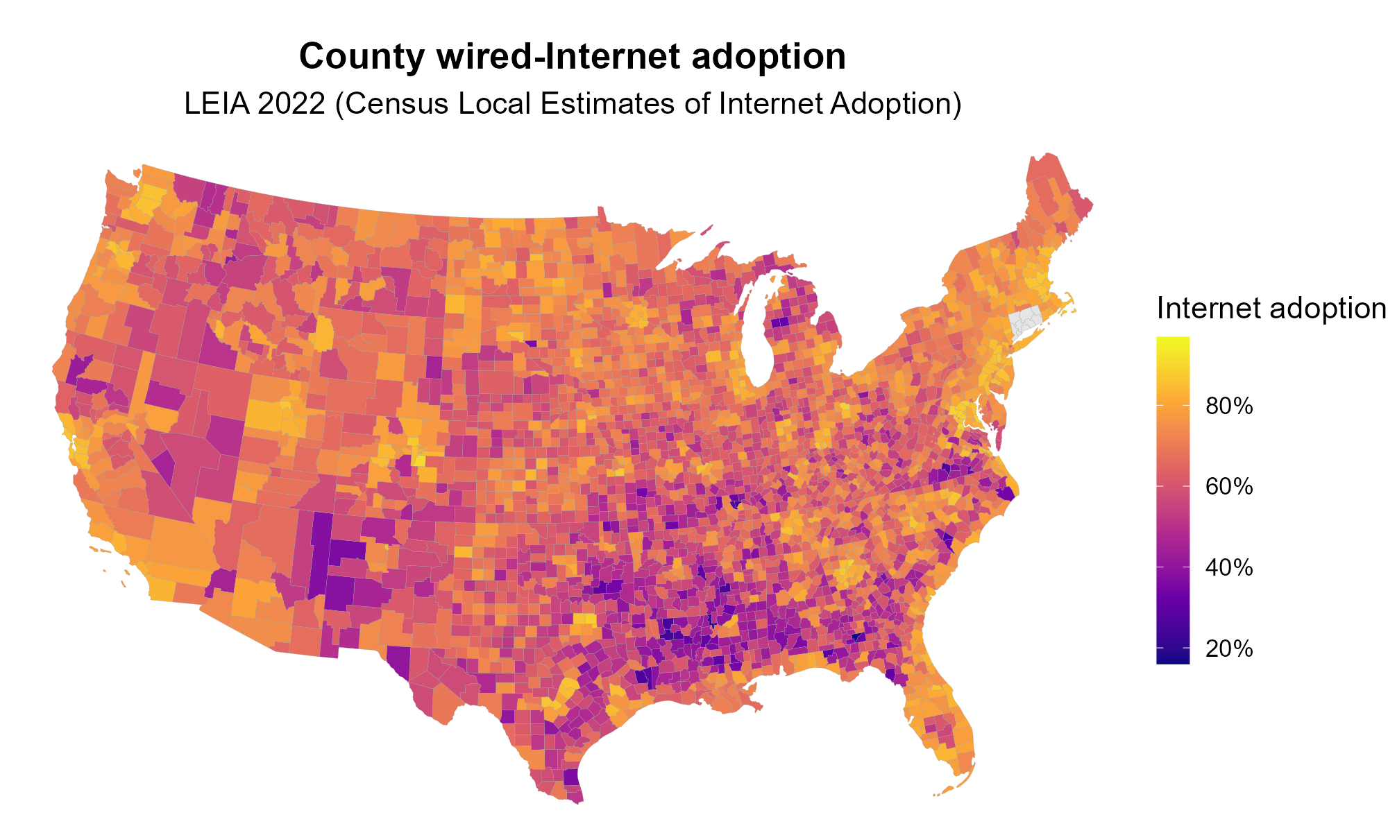
The heatmap below depicts adoption across 3,100 contiguous-U.S. counties. Differences are striking. Adoption ranges from 16.1 pp in the bottom-end Mississippi Delta and Appalachian counties to 96.8 pp in Seattle and D.C.; the median adoption rate across counties is 66.1 pp, while the interquartile range goes from 57.8 pp to 74 pp. This highlights that many counties have a significant share of households without wired internet at home.
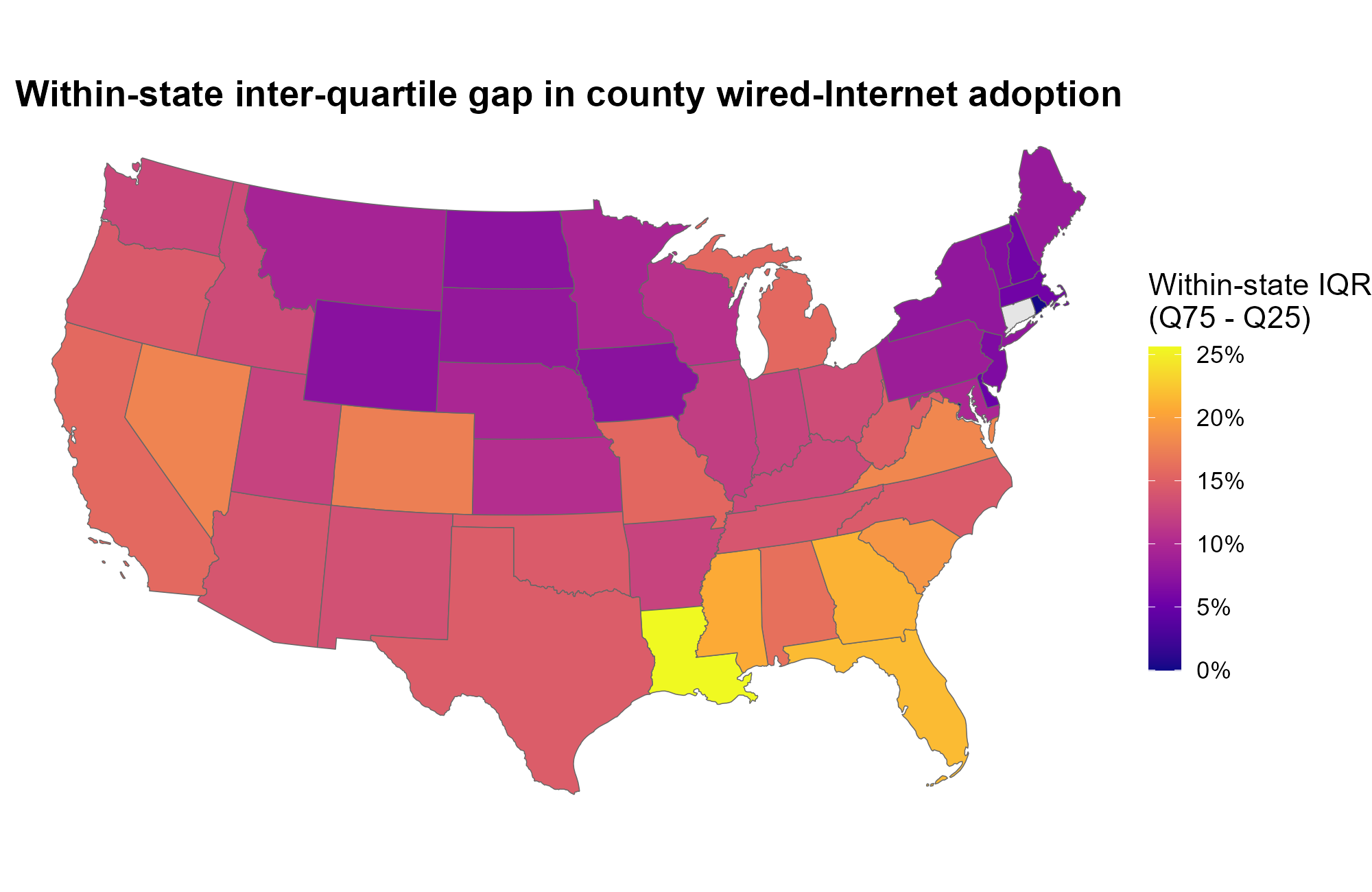
Differences within states are also substantial, especially in the South, where most low-adoption counties are concentrated. The figure below shows within-state inter-quartile ranges for adoption. The widest spread is within Louisiana, and is equal to roughly 25 percentage points (larger than the national inter-quartile range). Wide spreads are also present in Mississippi, Florida, and Georgia. The within-state spreads are narrowest in some Midwestern states, some of the Mountain States, and uniformly in the Northeast, which also has some of the highest adoption rates overall.
Local Factors Correlated with Differences Across Counties
A variety of county-level factors are correlated with lower adoption. While these relationships are not causal, they highlight a clear pattern: poorer, more rural areas with worse schools have lower adoption.
This is concerning because these are exactly the areas that stand to gain the most from high-quality home internet. Moreover, these are areas where people are less likely to have the means to pay for alternatives, such as satellite-based internet access (e.g., Starlink).
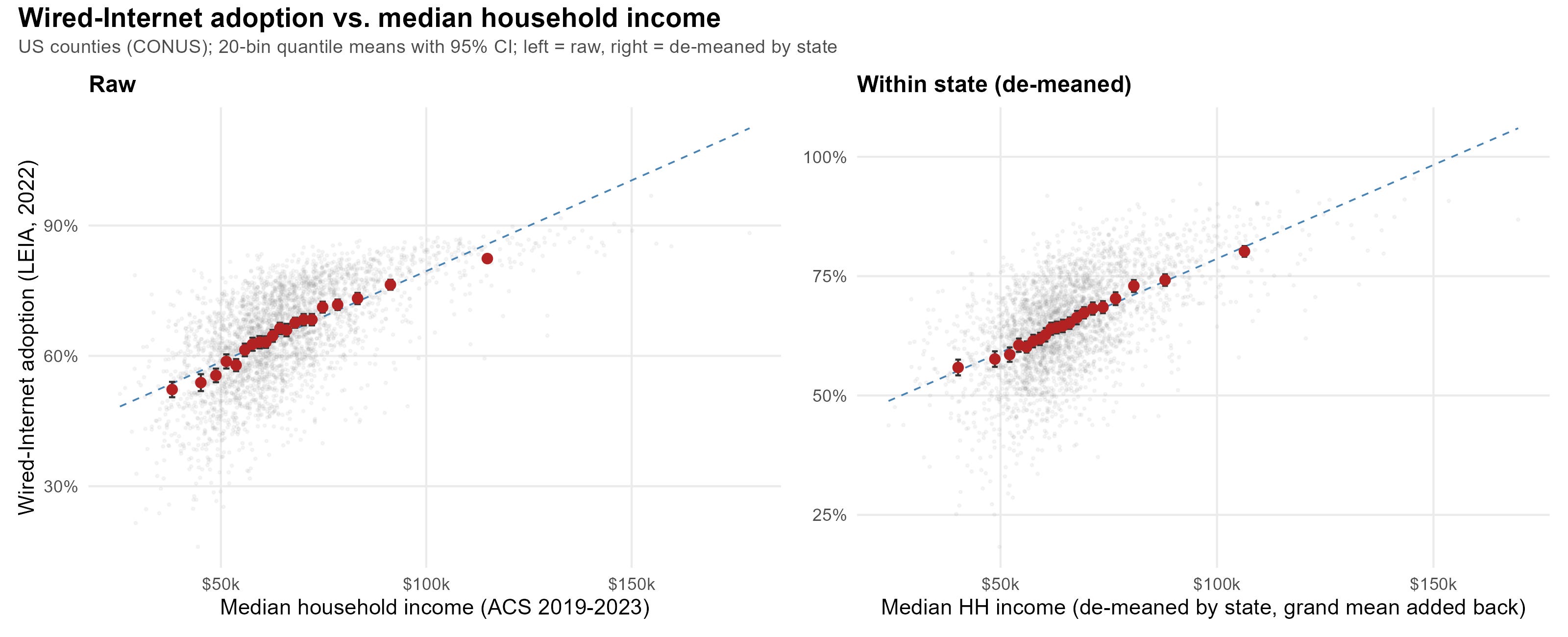
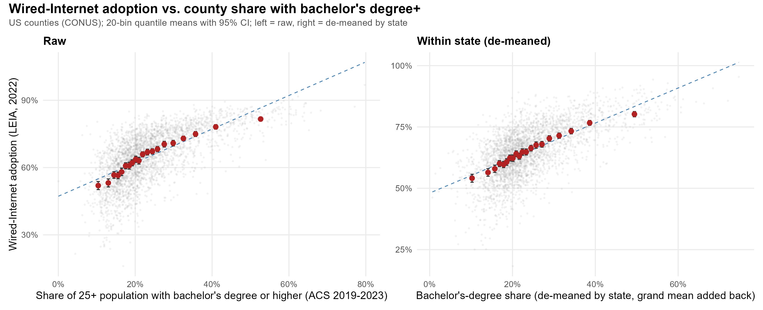
The scatterplots below depict the relation between wired-internet adoption and median income and between wired-internet adoption and the share of bachelor-educated individuals (strongly correlated with higher lifetime incomes). Both variables are from the 2023 American Community Survey 5-year estimates. The plots on the left show raw correlations across counties, while the plots on the right remove state means (fixed effects) and thus show within-state correlations. We restrict the sample to the continental U.S. (CONUS), to be consistent with the heatmaps above.
Adoption is strongly correlated with income, both across states and, most interestingly, within them. Adoption rises by 4.18 pp for every additional $10,000 in median income, and by 7.49 pp for every 10-percentage-point increase in the share of residents holding a bachelor's degree or higher.
While income and related proxies are the most straightforward variables to consider, we extend the analysis to two less conventional but equally important variables:
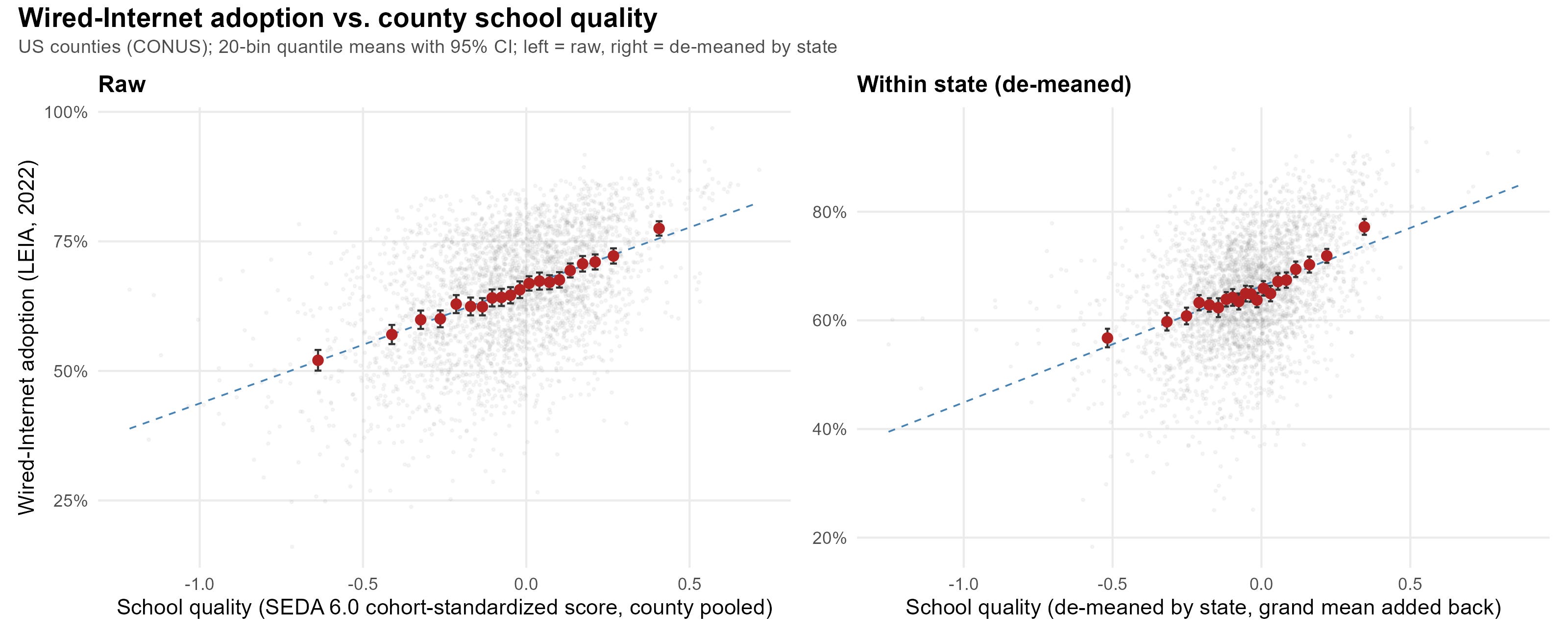
School quality: the Stanford Education Data Archive (SEDA) 6.0 cohort-standardized mean test score for each county (0 = national grade-cohort mean, +1 ≈ one SD above it).
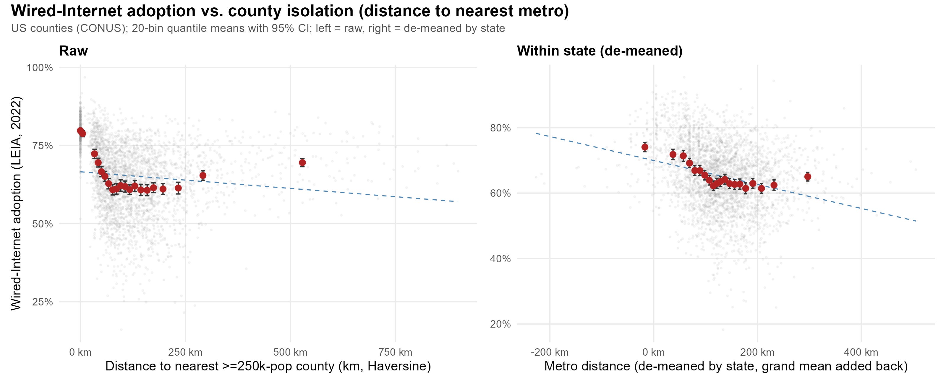
Isolation: the great-circle distance from each county’s centroid to the nearest county with 250,000+ people (median ≈ 101 km; we set this variable to zero for the large counties themselves).
We focus on these variables because they are good proxies for where access to remote services, information, and tools is likely to matter most. Online learning is more valuable where local schools are weak, and many services are harder to reach in places far from larger population centers or metropolitan areas.
For school quality (see the figure below), the raw relationship is strongly and monotonically positive: +22.65 percentage points of adoption per SD of school quality. The within-state version is very similar, with +21.46 pp per SD. This is particularly significant, since internet is a way to access educational tools and information. Low adoption likely amplifies the negative effects of lower-quality local education.
As for the isolation measure (see the figure below): looking across counties without state fixed effects, the gradient is mildly negative (−1.06 pp per 100 km) but strongly non-monotonic. Counties within ~50 km of a major metro have ~72–80% adoption; this drops sharply to ~61–62% across the 50–150 km band, then partially recovers to ~70% in the most remote bin. Adding state fixed effects yields a cleaner, steeper slope of −3.66 pp per 100 km.
Relation to School Quality After Demographic Controls
School quality is strongly correlated with demographic factors, which raises the question of whether its association with wired-internet adoption is just spanned by demographic differences. To test this, we run regressions with demographic controls and examine the coefficients on school quality and isolation. The controls include log median income, the share of residents with a bachelor's degree, the poverty rate, the share of residents aged 65 and over, and log total population, all drawn from the 2023 5-year American Community Survey. The table below reports the main results.
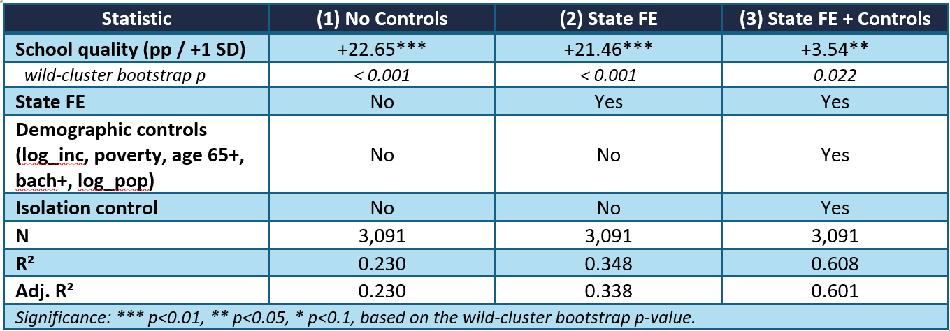
School quality survives every control. Even though the coefficient falls from +22.7 to +3.5 pp per SD as controls pile on, it stays significant throughout. A one-SD-better school score is still associated with 3–4 more points of adoption, conditional on income, education, age, poverty, county size, isolation, and state fixed effects.
Where the Gap is Most Concerning
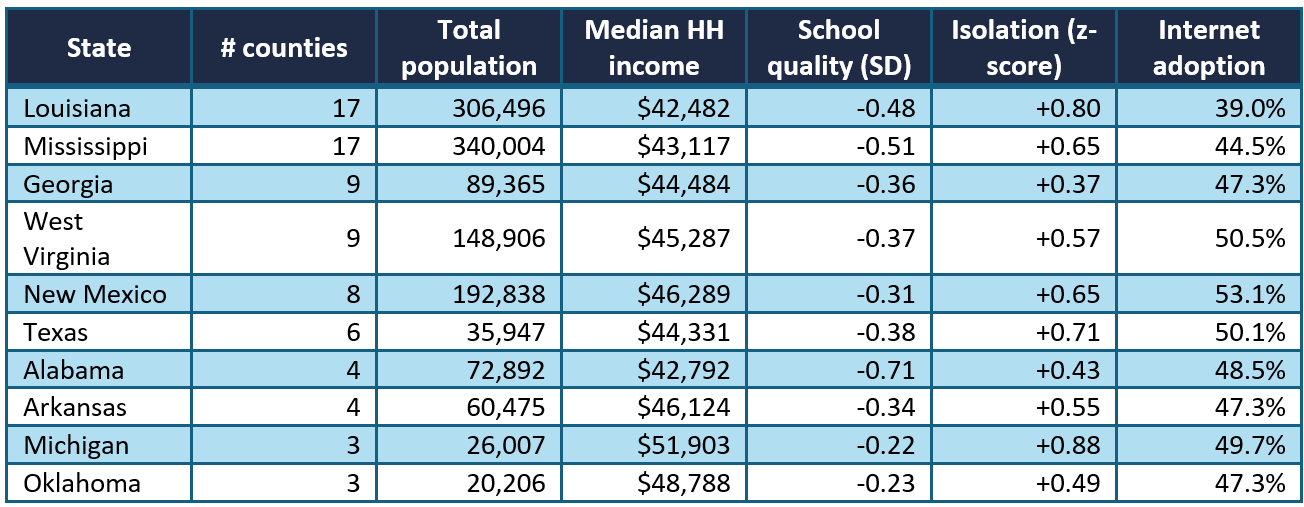
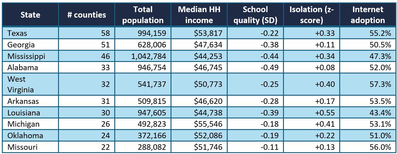
Let’s now consider the counties that fall simultaneously into the bottom quartile on income (≤ $54,901), the bottom quartile on school quality (≤ −0.191 SD), the top quartile on isolation (≥ 166 km), and the bottom quartile on wired-internet adoption (≤ 57.8%). This intersection contains 92 counties with a combined population of 1.54 million. The ten states with the most flagged counties account for 80 of the 92 counties and roughly 1.29 million of the 1.54 million residents in this set. The table below reports statistics for these 10 states, which are mostly located in the South. Adoption in these counties is very low: the mean falls below 40% in Louisiana, which also stands out for having the largest affected population and the weakest socioeconomic profile.
We repeat the exercise with median cutoffs: below-median income, below-median school quality, above-median isolation, and below-median adoption. This yields 506 counties across 40 states, with a combined population of about 9.68 million. The top ten states account for 353 of these counties and roughly 6.7 million residents. The list is still dominated by the South, though Texas, Georgia, and Mississippi now lead.
Conclusion
The county wired-internet gap is large; it is higher in lower-income counties and, even more concerningly, is tied to school quality and distance from major population centers. These relationships are also within-state, and the relation with poor school quality holds even after controlling for income, education, age, poverty, and size. Isolated counties with weak school districts would stand to gain the most from stable fast internet access, but they systematically have lower adoption.
One and a half million people live in counties that are in the worst quartile for income, schools, isolation, and wired-internet adoption at once. Almost 10 million people live in counties with below-median income, schools, above-median isolation, and below-median wired-internet adoption.
Our analysis shows that, despite the leading position of the U.S. in digital technology, internet services, and artificial intelligence, a substantial share of the population still lacks reliable access to these tools, and would benefit considerably from expanded wired connectivity or alternative technologies.