Multifamily Property Valuation Using Machine Learning

A Comparison of OLS Regressions and LightGBM for Multifamily Property Valuation in California.

Hedonic price regressions have long been the workhorse of commercial real estate research. In these models, the log of sale price is regressed on property and neighborhood characteristics using OLS, with fixed effects absorbing unobserved variation. These regressions are easy to implement and interpret: once coefficients are estimated from observed transactions, they can be combined with any property's characteristics to predict its valuation or expected sale price.

However, Koijen et al., 2025 show that this approach typically fits commercial real estate data poorly, unlike in the more liquid residential market, and yields noisy predictions. The same paper also shows that modern machine learning methods can substantially outperform traditional hedonic regressions in this setting.

In this post, we run a horse race between OLS and machine learning for a major commercial real estate segment: multifamily properties in California. Following Koijen et al. 2025, we use LightGBM as our machine learning method.

LightGBM is a decision tree method. A decision tree makes predictions by sorting observations through a series of yes/no questions until they land in a final group. For example, if you are predicting property prices, the tree might first ask “has this property more than 100 units?”. Then it might ask “is it in a high income neighborhood?” and so on. Each observation follows a path down the tree based on its characteristics until it reaches an endpoint, called a leaf. The predicted outcome for the observation is the average of the target variable (in our case, the property price) within the leaf.

We evaluate the LightGBM model along three dimensions: cross-sectional predictive accuracy, interpretability of the key valuation drivers, and susceptibility to overfitting. We find that the model substantially outperforms OLS in accuracy, while performing well on the other two dimensions.

Data and Estimation

We cover here the details of the data and estimation methodology. Readers interested primarily in seeing the results can skip ahead to the next section.

We collect a dataset of 12,177 arm’s-length sales of apartment buildings using data from Corelogic. We restrict the sample to buildings with at least 15,000 square feet of living area, spanning all 58 California counties from 2000 to 2025. We also collect neighborhood demographics from the American Community Survey at the Public Use Microdata Area level.

The dependent variable is the log of the sale price, demeaned by sale year to strip out aggregate time trends. Both the OLS and the LightGBM models compete purely on their ability to explain within-year price differences. The set of predictive features is identical for both: ten predictors covering building characteristics (log living area, log land area, log building age, and a “superstar county” indicator for Los Angeles, Orange, San Diego, San Francisco, San Mateo, and Santa Clara county), neighborhood demographics (population, elderly share, bachelor’s degree share, owner-occupied share, median income), and a CBSA market identifier.

The 12,177 observations are randomly divided into three non-overlapping sets: 60 percent for training (7,306 sales), 20 percent for validation (2,435), and 20 percent for the test set (2,436), which is used for the out-of-sample comparisons below. Note that the test set is never used in estimation. Year de-meaning is carried out using sale-year averages computed from the training set only, so that there are no information leaks from the validation or test sets.

The OLS model is estimated on the training set and its coefficients are applied to the test set covariates to generate predictions.

To explain how the LightGBM model is estimated, we begin by giving an intuition of how the model fits data. The LightGBM model starts with a naive guess, typically the unconditional mean of the variable it is trying to predict, which in our case is the log property price. It then looks at where the guess is wrong: for some observations it guesses too high, for others too low. A decision tree is built, splitting the data to try and predict these errors. The predictions of this tree are added to the original guess, scaled down by a factor (the learning rate) to avoid overcorrecting. The model then looks at the remaining errors, builds another tree to predict those, adds it in, and repeats. Each iteration of this process is called a boosting iteration.

LightGBM is estimated on the training set. Specifically, each boosting iteration runs estimates using a random subsampled of 70 percent of the training set, which decorrelates successive trees. At each boosting iteration, the Root Mean Squared Error is computed on the separate validation test, and the iteration with the lowest validation RMSE is selected for final prediction.

Readers experienced with non-parametric models may wonder how this validation-set approach compares to cross-validation. In a cross-validation approach, the model is estimated over multiple train-test partitions. LightGBM uses a fixed validation set for all boosting rounds, and an early-stopping routine (see below) to avoid overfitting. The downside relative to cross-validation is that performance estimates depend on a single random partition, but the benefit is computational efficiency and a clean separation between training set and evaluation set. Moreover, as mentioned, the model is re-estimated at every iteration on a different random subsample of the training set.

Both OLS and LightGBM forecasts are produced in the de-meaned space and then converted back to the original log price scale by adding the training set year means, so that RMSE and R-squared are directly comparable across models. Thus, the horse race between the models is based on their ability to predict prices across properties at a point in time.

All results below come exclusively from the held-out test set, and so are actual out-of-sample predictions.

LightGBM Wins on Out-of-Sample Predictions

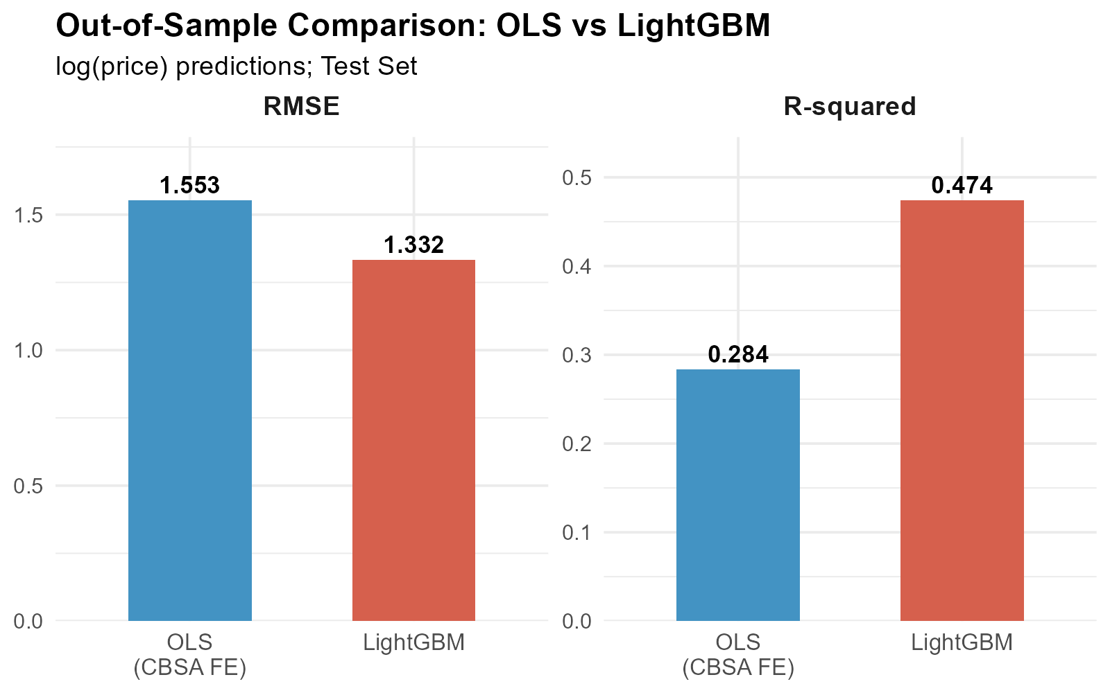
On the held-out test set, LightGBM achieves a test RMSE of 1.332, which is roughly 14 percent lower than the OLS test RMSE of 1.553. In R-squared terms, LightGBM explains about 47 percent of out-of-sample price variation versus 28 percent for OLS. This is a gain of nearly 19 percentage points (close to a 70% relative improvement). Same features, same data, same year de-meaning. The improvement comes entirely from LightGBM’s ability to capture non-linear relationships and feature interactions.

A caveat: these absolute R-squared values are modest compared to single-family hedonic models, which often exceed 0.90. However, multifamily apartment buildings (and commercial real estate more broadly) are inherently harder to value due to fewer transactions and greater variation in asset characteristics. This challenge is compounded by the limited set of hedonic variables available for our analysis.

What Drives LightGBM Predictions?

A common knock-on of machine learning models is the “black box” problem. What drives predictions? Are the estimates sensible?

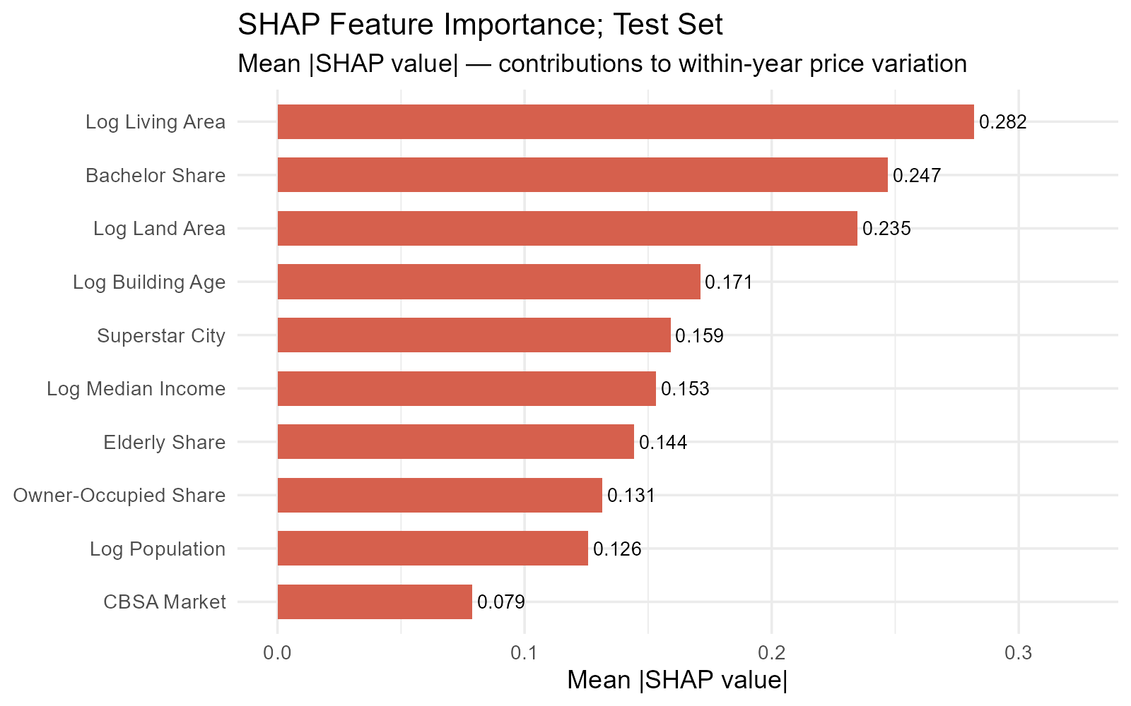
The analysis of SHAP values helps address this concern. For every test observation, SHAP decomposes the model’s prediction into additive contributions from each predictive feature. Averaging the absolute SHAP values across the test set gives us a global importance ranking, indicating which features are most important for prediction.

The top three features are log living area (mean |SHAP| = 0.282), bachelor’s degree share (0.247), and log land area (0.235). Building size is, unsurprisingly, the single strongest predictor. The prominence of the bachelor’s degree share is interesting. It proxies for neighborhood quality and tenant demand in an intuitive way. Areas with more educated residents tend to have higher rents and lower vacancy, both of which are capitalized into property values.

Log building age (0.171) and the superstar-city indicator (0.159) follow, capturing the age discount and the persistent price gap between California’s expensive coastal counties and the rest. Median income, elderly share, owner-occupied share, and population fill the middle ranks. The CBSA market identifier comes in last (0.079): most of the metro-level variation is already absorbed by the demographic features and the superstar indicator.

What about the direction of heterogeneity? What is the sign of the effect of each feature on prices? A Beeswarm plot shows this: each dot represents one observation; its horizontal position indicates the SHAP value, and its color encodes the actual feature value (blue = low, red = high). A feature that has predominantly red dots to the right and blue dots to the left has a positive effect on prices (higher values of the feature, higher prices).

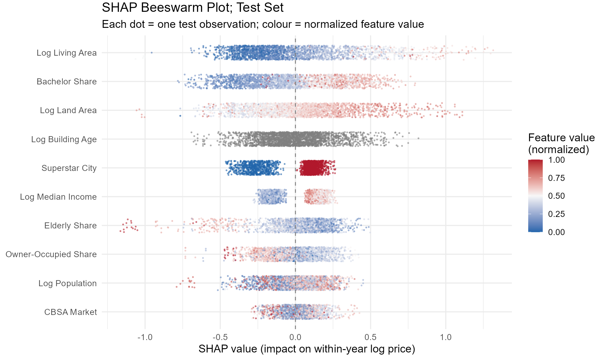
Log living area shows a clean, positive gradient: larger buildings raise predicted prices, while smaller ones lower them. The spread is wide, confirming that building size drives the largest swings at the observation level.

Bachelor’s degree share displays similarly clean color separation. Neighborhoods with more college-educated residents receive positive SHAP contributions; those with low attainment receive negative ones. The effect is nearly monotonic, reinforcing that neighborhood human capital is a robust price driver.

Log building age is notably different. The relationship is noisy and non-linear. This is exactly the kind of complex pattern that tree-based models handle naturally but a log-linear OLS specification cannot.

The superstar-city indicator splits into two clusters, as expected from a binary variable. Properties outside the six superstar counties show a tight band of negative SHAP values, while those inside cluster around a positive contribution.

Across demographics, median income shows a clear positive gradient, whereas the elderly share shows the opposite: neighborhoods with large elderly populations are associated with lower apartment building prices.

Overfitting?

None of this matters if LightGBM is just memorizing training data. Several guardrails keep the model reliable. A conservative learning rate of 0.05 means each new tree contributes only five percent of its prediction to the running total. Trees are kept shallow (max 20 leaves, and a maximum of 8 levels of depth), and every leaf must contain at least 300 observations. Moreover, training is run at each iteration on a different subsample of the training set.

The most important safeguard is early stopping. At every boosting iteration, RMSE is evaluated on the validation set. If 100 consecutive rounds pass without improvement, training halts. The final predictions use the best-performing iteration, not the last one.

The best iteration in our exercise was round 2,208, with a moderate gap between training and validation error.

Conclusion

For multifamily property valuation, LightGBM delivers a meaningful improvement over OLS in out-of-sample performance, with 14 percent lower prediction error and 19 extra percentage points of explained variance, without sacrificing interpretability.

Does this mean we should throw out hedonic regressions? Not at all. OLS remains a useful, interpretable benchmark and, when combined with causal variation, can offer clear insights into what affects real estate prices.

However, when the goal is pure prediction (i.e., forecasting what a property will sell for), machine learning is a powerful tool that can improve on OLS.